Loading content...
Table of Contents
Back to all internships
Data Engineering Internship
Oeson
Indore, India
November 2025 - February 2026
PythonDatabricksPandasETLGoogle ColabApache AirflowPower BIMicrosoft FabricDAXDelta LakePySpark
Overview
Completed a 3-month Remote Data Engineering Traineeship and Internship with Oeson, where I learnt about the three layered architecture in Databricks, Apache Airflow for 8 weeks and a 4 week final internship project where I had to choose 1 out of 4 projects.
Experience Details
Overview
Completed a 3-month Remote Data Engineering Traineeship and Internship with Oeson, where I learnt about the three layered architecture in Databricks, Apache Airflow for 8 weeks and a 4 week final internship project where I had to choose 1 out of 4 projects.
Experience Details
In the Final 4 weeks of this internship, I was allowed to choose between 4 Data Engineering projects:
Project Options
Available Projects
- End-to-End ETL Pipeline for Healthcare Appointment No-Show Analytics (Bronze → Silver → Gold)
- HR Attrition Analytics ETL Pipeline (Bronze → Silver → Gold)
- Energy Consumption ETL Pipeline (Bronze → Silver → Gold) for Smart Household Analytics (Selected)
- End-to-End ETL Pipeline for UK Road Accident Analytics (Bronze → Silver → Gold)
Selected Project: Energy Consumption ETL Pipeline
I chose the Energy Consumption ETL Pipeline for Smart Household Analytics because of its complexity and the ability to extend this project and make a machine learning demand forecasting model on the data.
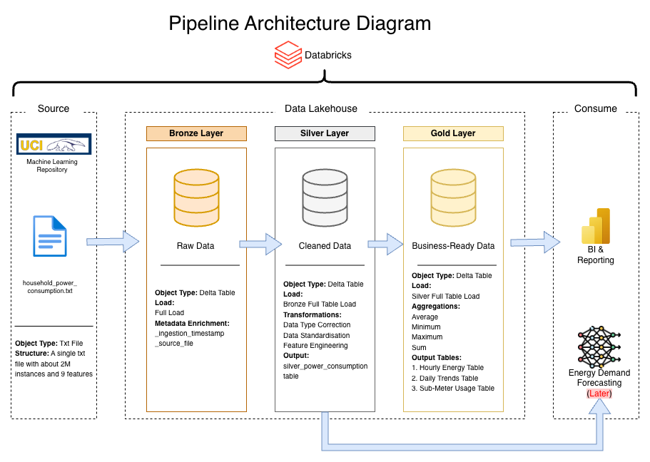
Pipeline Architecture
In the Consume section, I decided to use Power BI because of an interview for a role where I got to understand how Power BI is been used to host the semantic models of the company's data after it has been processed with Snowflake. This made me curious to see if I could implement the same using Databricks. This was a nice addition to make the analysis and visualization because Databricks' built in a visualization tool has fewer features compared to Microsoft Fabric Power BI's maturity.
After processing the data in Databricks, I connected directly to my Delta tables through Microsoft Fabric's Lakehouse architecture to build an interactive business intelligence dashboard.
Links
Data Engineering & Visualization
What This Project Does
This project takes raw electricity usage data from a smart meter system and processes it through three stages: Bronze: Store raw data as-is, Silver: Clean and organize the data, Gold: Create summary tables for analysis. The goal is to help an energy analytics team understand when and how electricity is being used in a household.
The Data
Source: UCI Machine Learning Repository - Individual Household Electric Power Consumption. Size: Over 2 million rows of minute-by-minute data.
Environment Setup
File: config/setup.ipynb - This notebook initializes the ETL infrastructure and must be run first. It creates catalog (energy_demand_catalog), schema based on selected environment (dev or prod), creates volume for file storage, defines table names and full paths for all layers, and storage paths for data and checkpoints.
Bronze Layer
File: notebooks/01_bronze.ipynb - This layer downloads the raw data file and stores it without changes. It downloads ZIP file from the UCI website, extracts the text file, reads it with semicolon separators, adds metadata columns (_ingestion_timestamp, _source_file_name), and saves as a Delta table. Output: energy_demand_catalog.{env}.raw_power_usage
Silver Layer
File: notebooks/02_silver.ipynb - This layer cleans and prepares the data for analysis. Cleaning steps: Combines Date and Time columns into one datetime column, converts numbers from text to decimal format, replaces missing values ("?") with empty values, removes rows with bad timestamps, filters out negative power readings, renames columns to lowercase with underscores.
Sub-meter Unit Conversion: Sub-meter values were converted from Wh to kWh (divided by 1000). New columns added: hour_of_day, day_of_week, is_weekend, consumption_kwh. Output: energy_demand_catalog.{env}.silver_power_consumption
Gold Layer
File: notebooks/03_gold.ipynb - This layer creates three summary tables for business analysis.
Table 1: Hourly Summary
Name: agg_hourly_metrics - Shows average usage patterns by hour of day: hour_of_day, avg_consumption_kwh, min_voltage, max_voltage, avg_current_intensity. Purpose: Find which hours of the day use the most electricity.
Table 2: Daily Summary
Name: agg_daily_metrics - Shows daily totals and patterns: date, total_kwh, avg_kwh, peak_hour, weekend_flag. Purpose: Compare weekdays to weekends and track daily trends.
Table 3: Sub-Meter Summary
Name: agg_submeter_metrics - Shows daily totals by area of the house: date, sub_meter_1_total (kitchen), sub_meter_2_total (laundry), sub_meter_3_total (water heater and AC). Purpose: See which parts of the house use the most energy.
Project Files
energy-demand-etl/ ├── config/ │ └── setup.ipynb ├── notebooks/ │ ├── 01_bronze.ipynb │ ├── 02_silver.ipynb │ └── 03_gold.ipynb ├── docs/ │ └── internship_architecture.drawio.svg └── README.md
Final Outcome Of Pipeline
After running all notebooks, you will have: 1. Four Delta tables in Databricks: raw_power_usage (bronze), silver_power_consumption (silver), agg_hourly_metrics (gold), agg_daily_metrics (gold), agg_submeter_metrics (gold). 2. Cleaned data CSV exported to your volume storage. 3. Sample outputs displayed in the Gold notebook.
Future Extensions
- Demand forecasting models
- Anomaly detection for unusual consumption patterns
- Integration with smart home systems for automated energy management
Outcome & Key Achievements
Built complete ETL pipeline and Power BI dashboards with 17.9% weekend variance insight